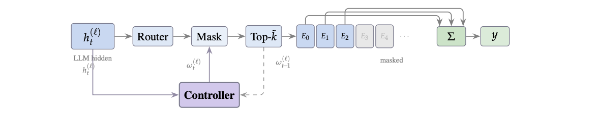
Temporally Extended Mixture-of-Experts Models

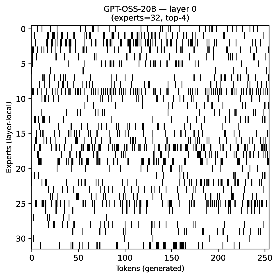
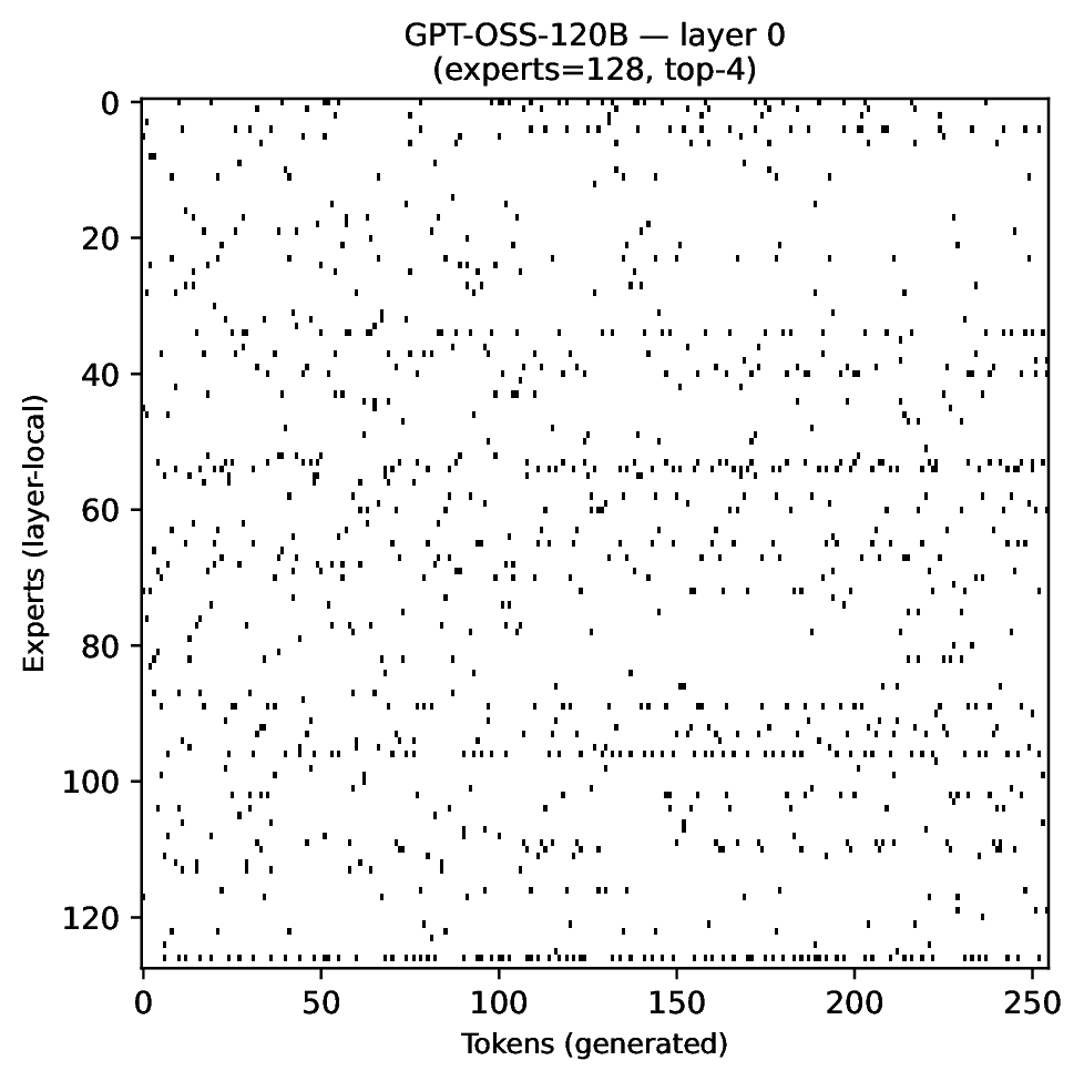
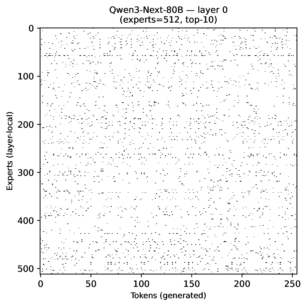
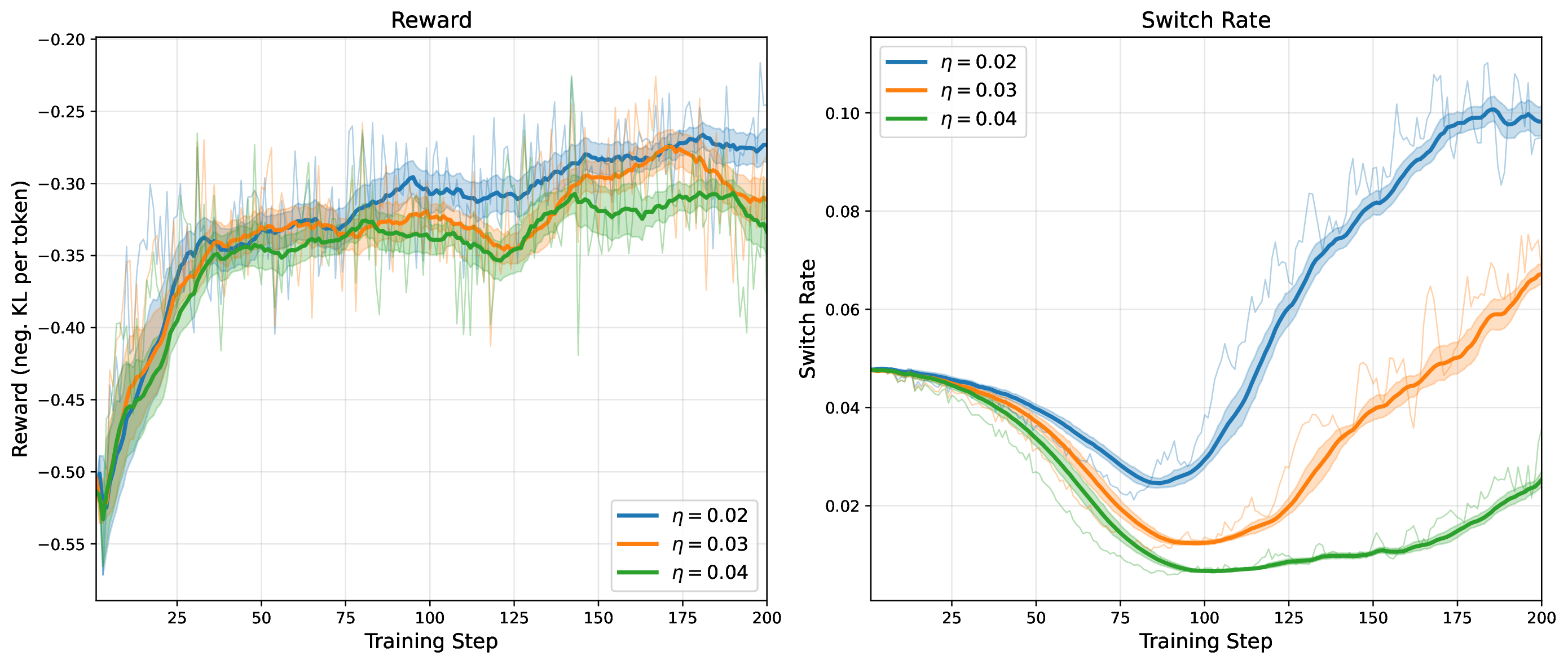
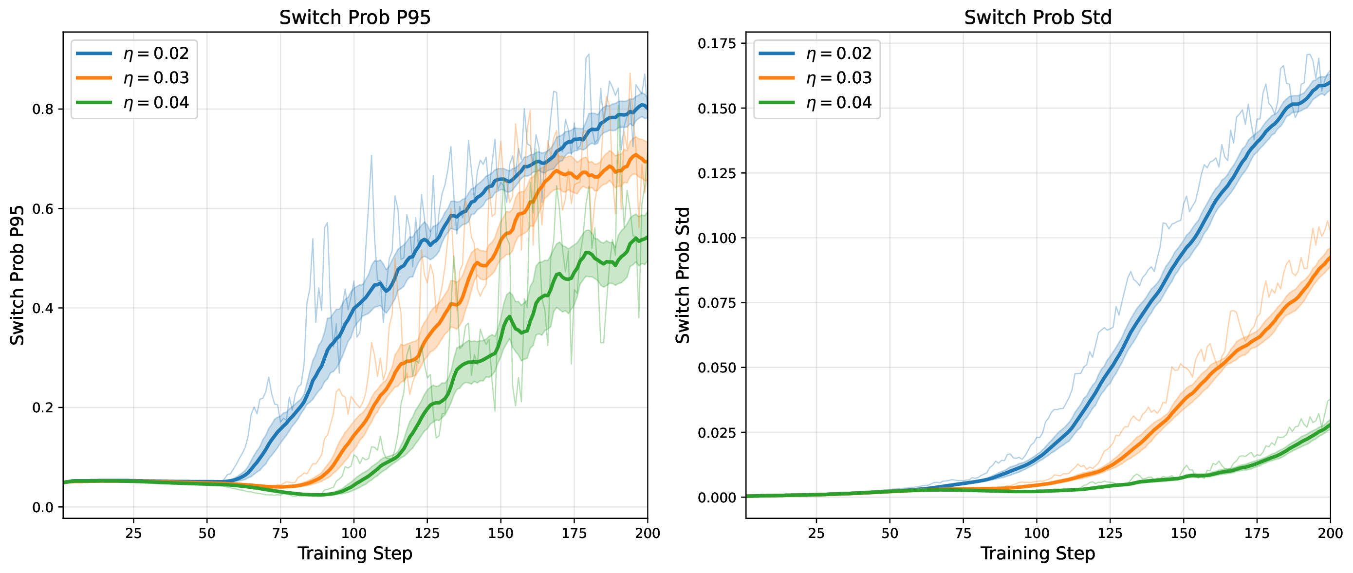
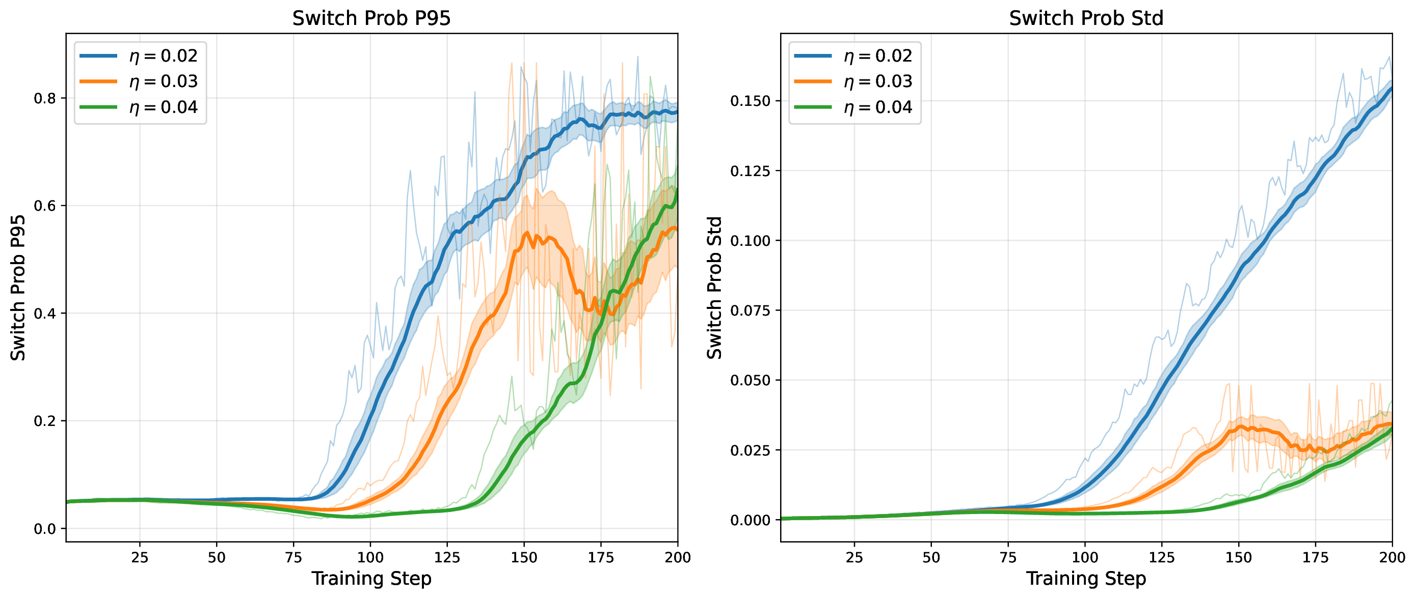
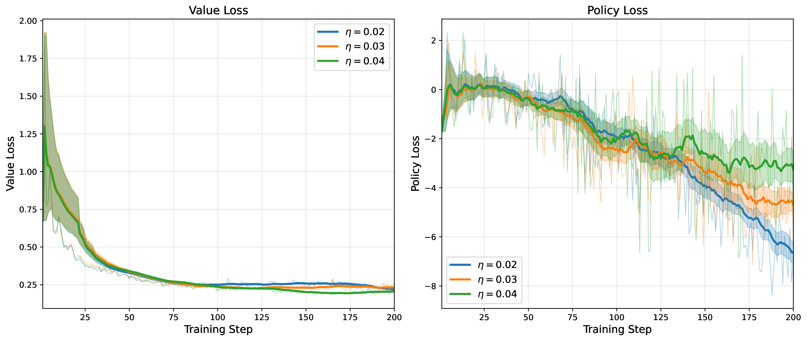
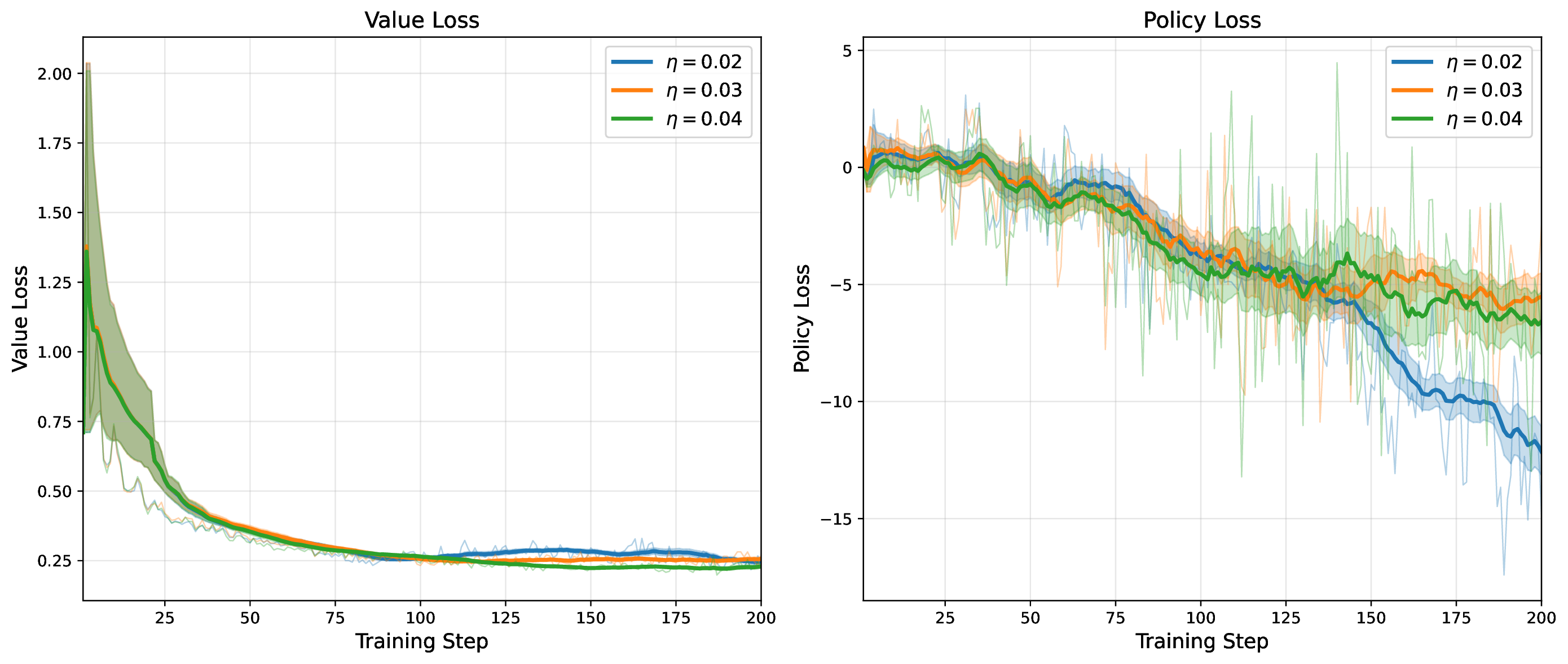
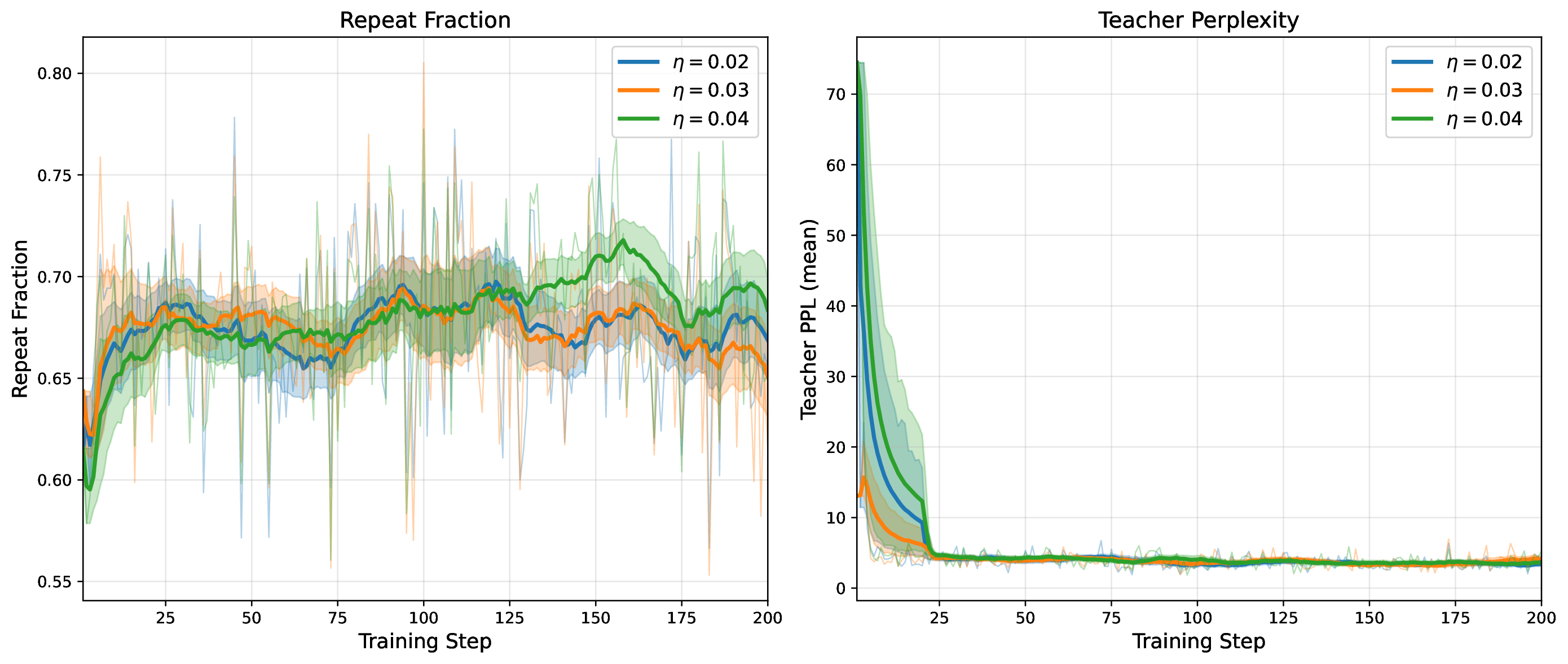
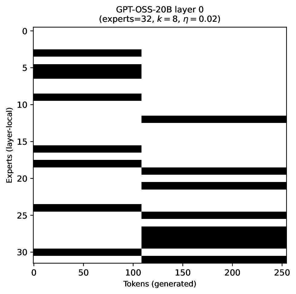
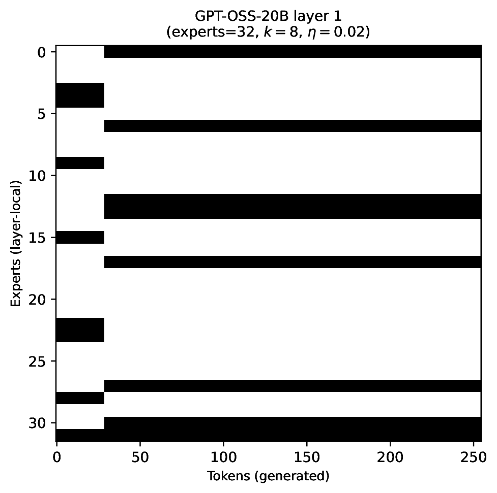
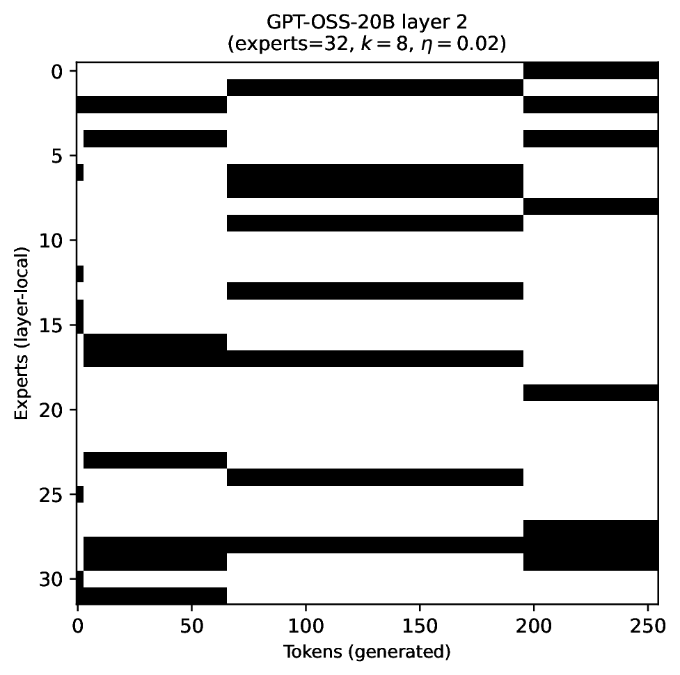
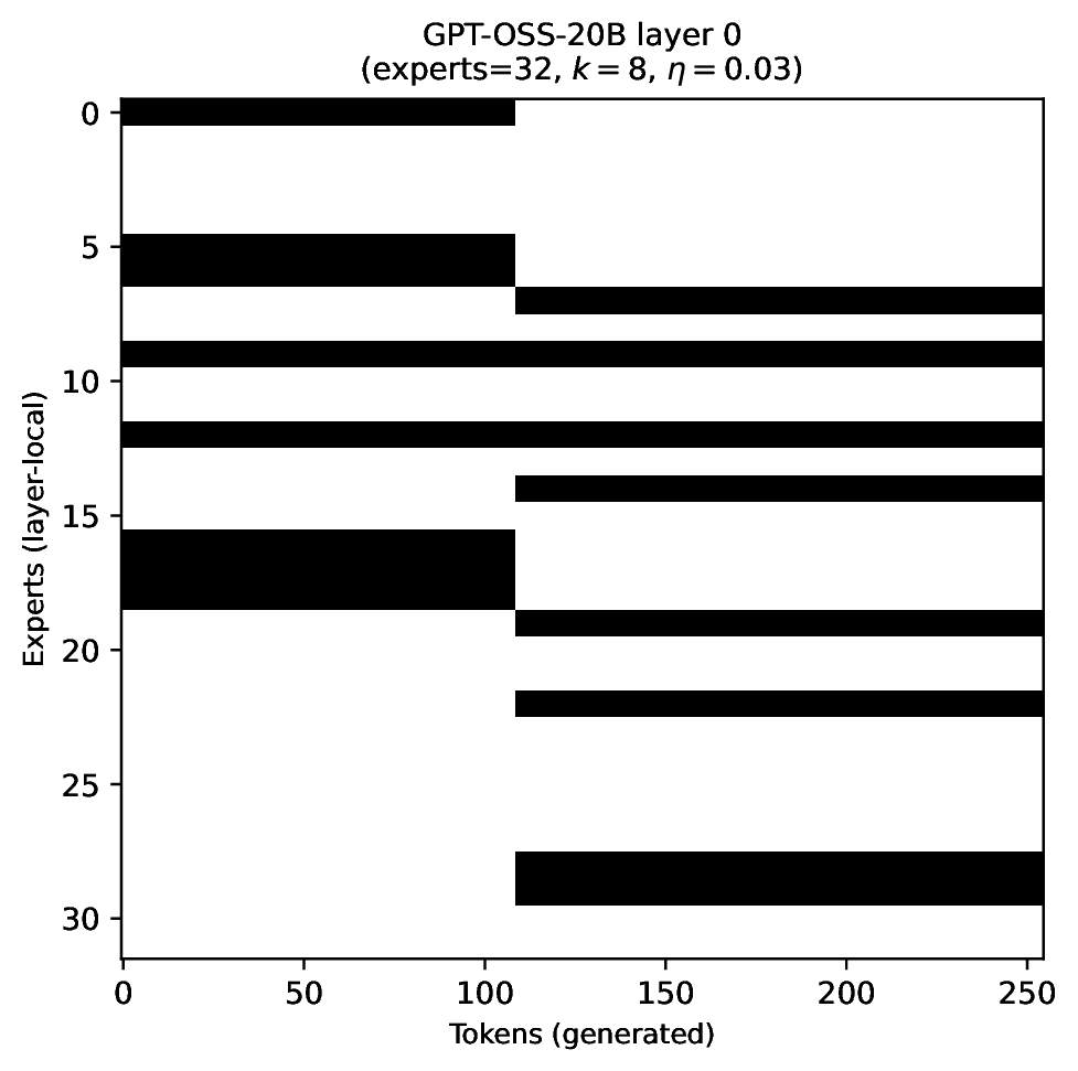
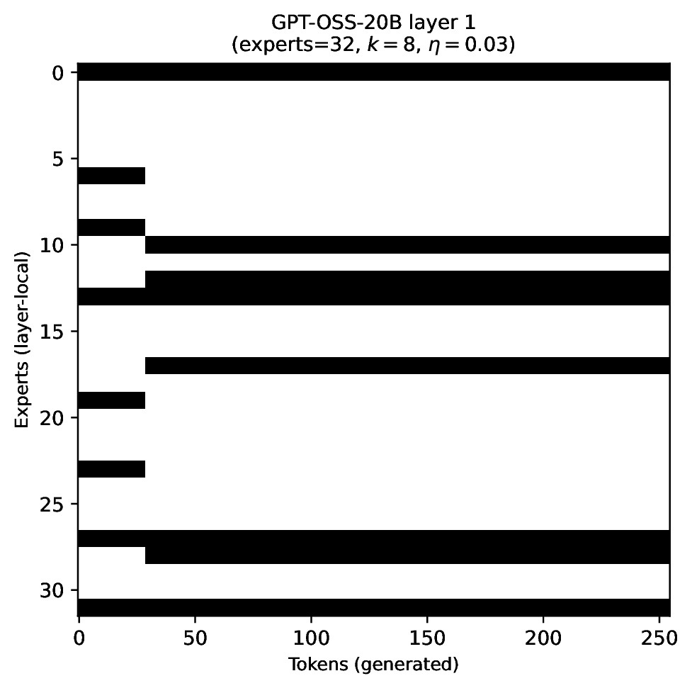
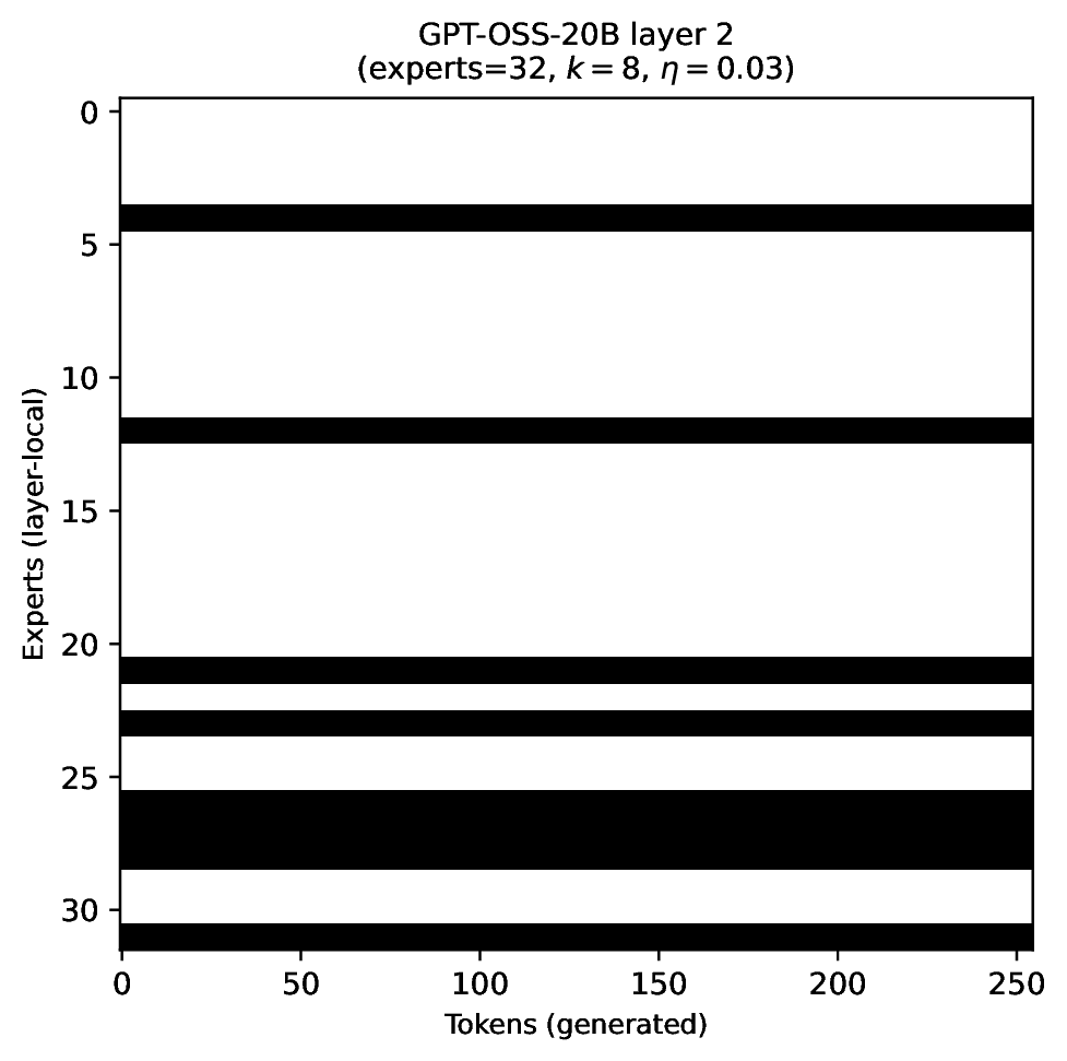
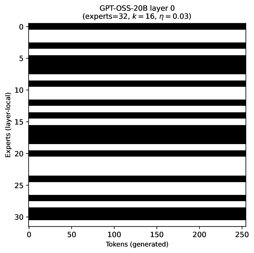
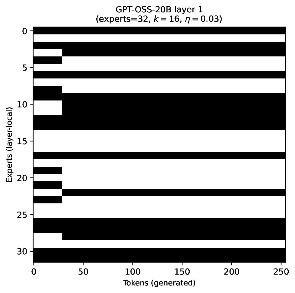
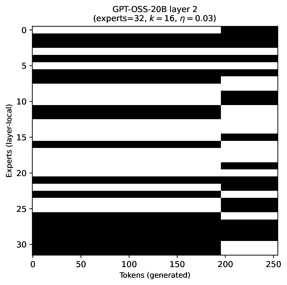
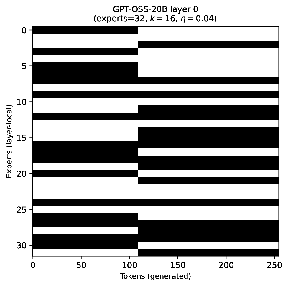
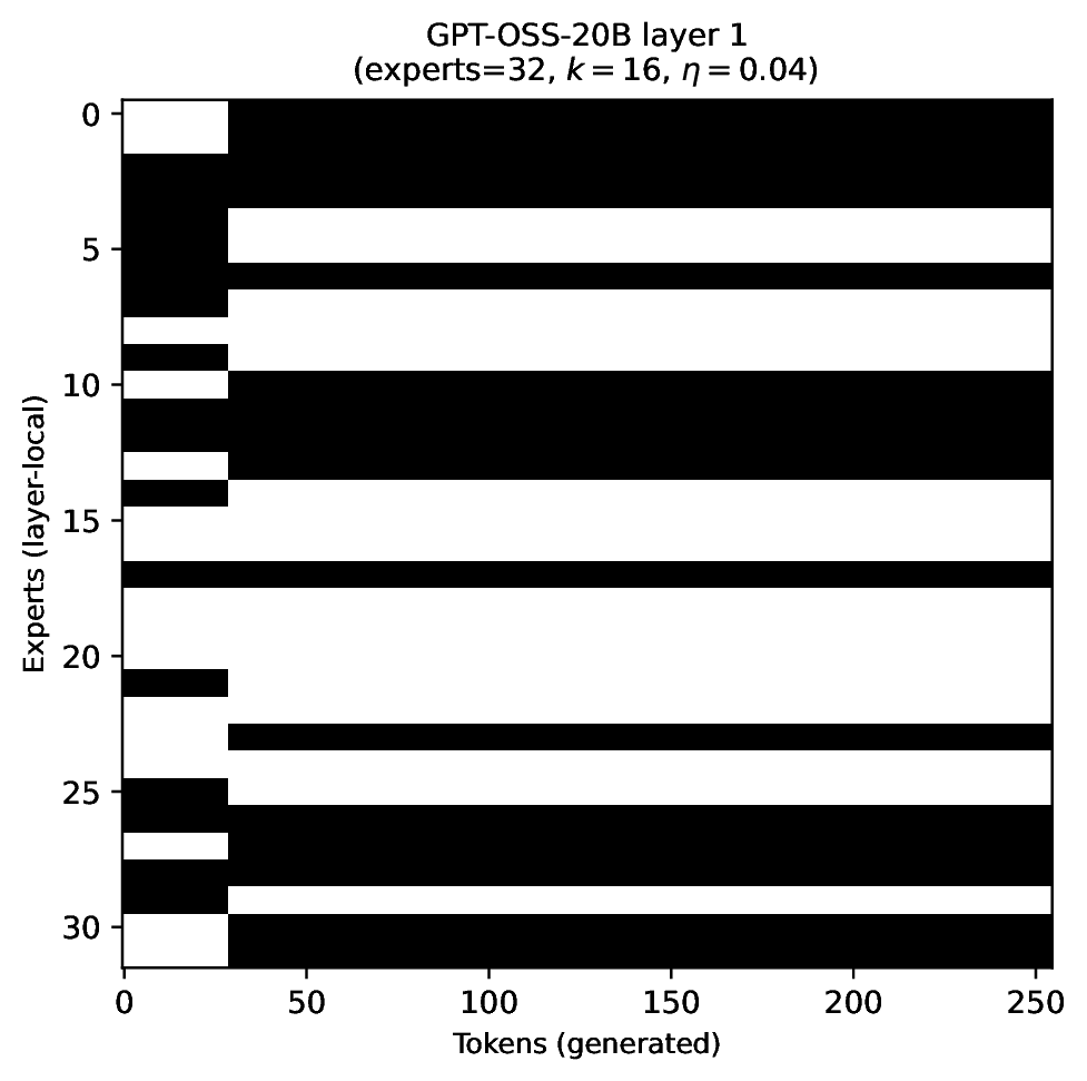
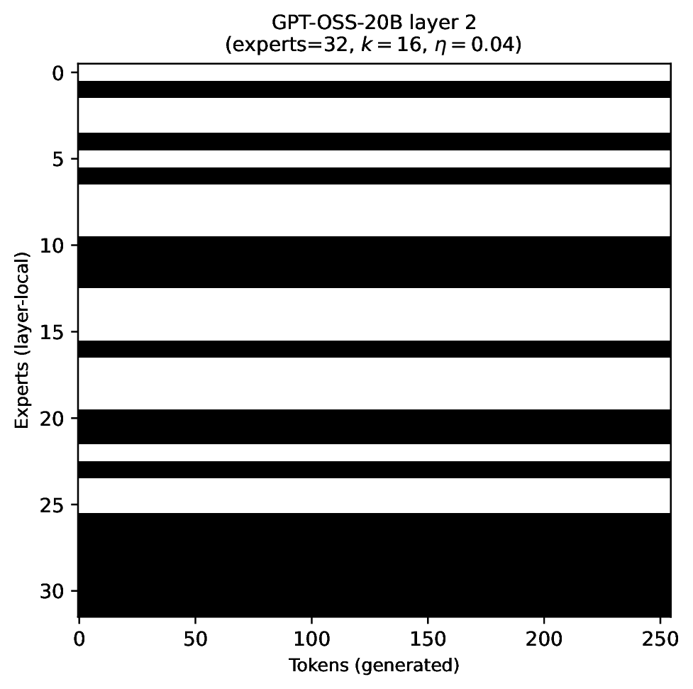
Modern MoE LLMs switch their active expert set at almost every generated token. That foreclosures memory optimizations like offloading once expert counts outgrow GPU capacity. We argue that this is exactly the structure that options with deliberation costs were designed for — and show that even pretrained MoEs (like gpt-oss-20b) can be cheaply converted into temporally extended ones, dropping switch rates from >50% to under 5% while retaining most of the base model's accuracy.

Zeyu Shen, Peter Henderson

Princeton University

PDF Code

Standard MoE switches experts every token; our temporally extended controller learns to keep the same expert set for many tokens at a time, enabling memory-efficient serving, temporal chunking for training, and expandable continual learning.

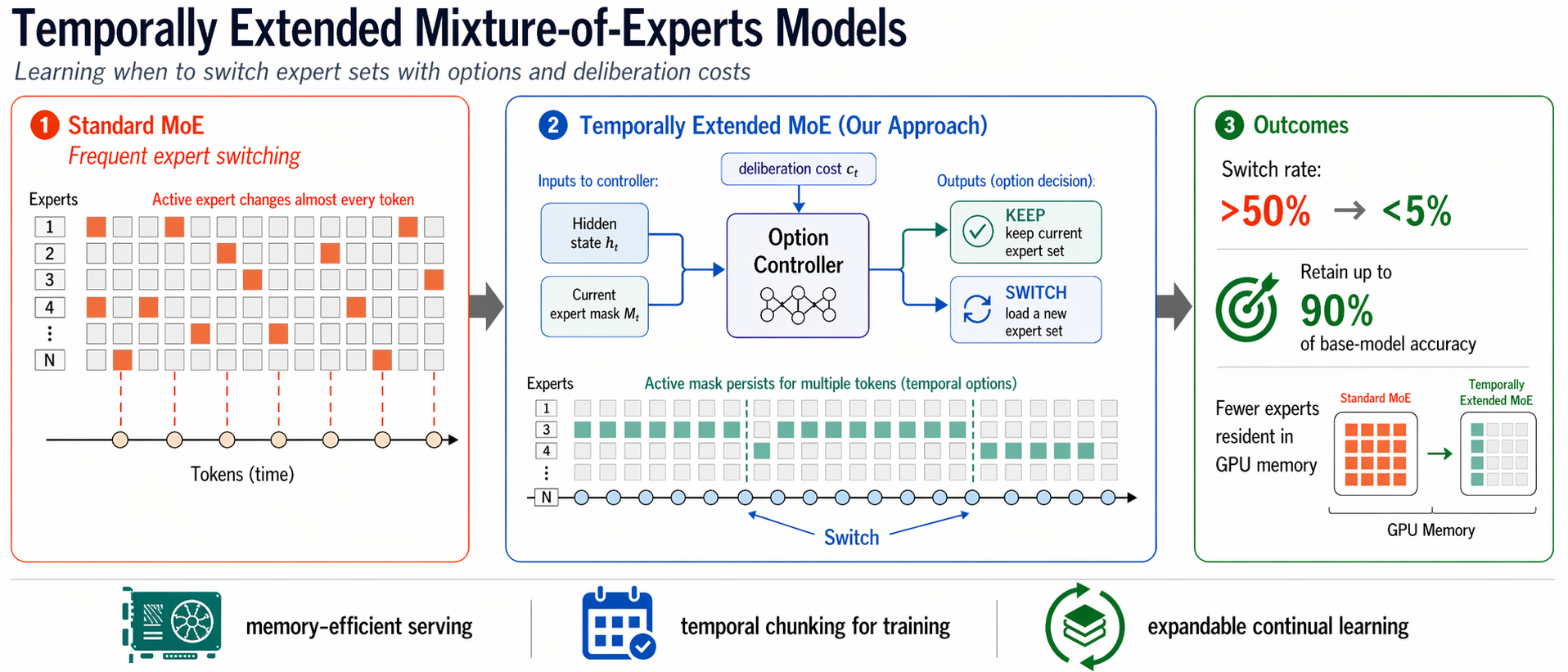
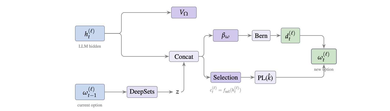
Standard MoEs change their active expert set at almost every token. Our option controller learns when to keep the current set and when to switch, governed by a deliberation cost η. The result: switch rates collapse from over 50% to below 5%, while accuracy stays close to the base model — opening the door to memory-efficient serving, temporal chunking for training, and continual expansion of the expert pool.

The Problem: MoE Routing Has No Temporal Structure

Mixture-of-Experts (MoE) layers are everywhere in modern LLMs — Gemini-2.5-Pro, DeepSeek-V3, Qwen3-Next-80B, gpt-oss, and many more. Only a sparse subset of experts is active per token, so a 120B-parameter model like gpt-oss-120b only activates ~5B parameters at a time. In principle, you can keep growing the expert pool while inference compute stays flat.

But once the experts no longer fit on GPU, weights have to live on host memory or disk and be loaded on demand. Every load is latency. Current MoE routers don't account for this cost at all: the active expert set changes at almost every token. We measured this directly across three frontier open-source MoEs, on 1,000 prompts spanning chat, code, math, STEM, and 6 multilingual categories — the switch rate is essentially 1.

gpt-oss-20b — layer 0

gpt-oss-120b — layer 0

Active experts vs. token position, Qwen3-Next-80B layer 0

Qwen3-Next-80B-A3B — layer 0

Active experts (rows) over generated token positions (columns) on the same prompt. There is essentially no temporal structure: nearly every column is a fresh draw.

See the per-category switch rate table

Average switch rate across 100 prompts per category (with $\maskk = \activek$, i.e., the model's native top-$\activek$). Mean ± std.

Model	Chat	Code	Math	STEM	Multi (en)	Multi (de)	Multi (es)	Multi (fr)	Multi (it)	Multi (ja)
gpt-oss-20b	0.94	0.95	0.94	0.95	0.95	0.95	0.95	0.95	0.95	0.95
gpt-oss-120b	0.98	0.99	0.99	0.99	0.99	0.99	0.99	0.99	0.99	0.99
Qwen3-Next-80B	1.00	1.00	1.00	1.00	1.00	1.00	1.00	1.00	1.00	1.00

Why this matters: missed opportunities

If the active expert set were temporally extended, several memory-related optimizations become natural:

Inference serving with reduced memory. Only the $\maskk$ active experts need to be GPU-resident; the other $N - \maskk$ can stay on host or disk. For gpt-oss-20b, keeping 16 of 32 experts saves ~4.7 GiB (37%); keeping 8 saves ~7.1 GiB (55%) of VRAM.
Memory-efficient training via temporal chunking. Each contiguous chunk of tokens can be associated with a fixed expert mask, so only those experts participate in the forward and backward pass. Inactive experts can be offloaded for the chunk.
Continual learning with expandable expert capacity. Because only $\maskk$ of $N$ experts are active at a time, you can keep adding experts (e.g., to adapt to new domains) without growing the per-token compute or active memory footprint.

The Idea: MoE Routing as Options With Deliberation Costs

Choosing when to commit to a set of resources and when to pay the cost of switching is exactly the structure formalized by temporally extended actions in the options framework (Sutton, Precup, Singh, 1999). An agent picks a high-level "option" that persists over many time steps; switching to a new option incurs a deliberation cost (Harb et al., 2018).

We propose temporally extended Mixture-of-Experts: a small per-layer controller that learns when to switch the expert set and which one to switch to, optimized via the option-critic architecture (Bacon et al., 2017) augmented with a deliberation cost η. Because the switching cost is an explicit term in the objective, the controller automatically discovers temporal structure — it only switches when the expected quality gain justifies the cost.

Cast as

s-MDP with options

Each layer's expert mask is an option $\omega^{(\ell)}_t$; expert loading latency is the deliberation cost.

→

Add
Lightweight per-layer controller
Termination head, value & option-value heads, and a Plackett–Luce selection head. Initialized from the router; trained with option-critic + deliberation cost.

→

Train via

Self-distillation

Reward is per-token reverse KL between the (frozen) base model and the controller-augmented student. LoRA on experts & attention, full grads on router.

The intra-option policy is the LLM itself; primitive actions are generated tokens. Critic and termination updates follow A2OC (Harb et al., 2018) with GAE($\lambda$); intra-option policy gradients use Monte Carlo returns.

How It Works

Per-layer pipeline: hidden state goes to the router; the router's top-k is restricted to the active mask, those experts run, and outputs are summed. The controller produces the mask from the hidden state and the previous mask. — Per-layer view. The router's top-$\activek$ is restricted to the active mask $\omega^{(\ell)}_t$, so only the experts in the mask contribute; the rest are skipped. The controller (purple) sets that mask from the hidden state $h^{(\ell)}_t$ and the previous mask $\omega^{(\ell)}_{t-1}$.

Options formulation

For each MoE layer $\ell$, the option space is the set of binary expert masks of size $\maskk$:

$$\Omega^{(\ell)} = \big\{\omega \in \{0,1\}^N : \|\omega\|_1 = \maskk\big\}.$$

The router is constrained to pick its top-$\activek$ experts only from the active mask $\omega^{(\ell)}_t$. The mask persists across tokens until a termination decision $d^{(\ell)}_t = 1$ triggers selection of a new mask. We factorize across layers for tractability: each layer has its own controller conditioning on its hidden state and current mask.

Controller architecture

Each MoE layer gets its own controller, operating on the pre-MLP hidden state $h^{(\ell)}_t$ and the current mask $\omega^{(\ell)}_{t-1}$. It has four heads:

Expert-set embedding. A DeepSets encoder $z^{(\ell)}(\omega) = \tfrac{1}{\maskk}\sum_{i \in \omega} \varphi(e_i)$ over learned per-expert embeddings produces a permutation-invariant representation of any mask.
Termination head. $\beta^{(\ell)}_t = \sigma\big(\mathrm{MLP}_\beta\big(\overline h^{(\ell)}_t,\, \overline z^{(\ell)}(\omega^{(\ell)}_{t-1})\big)\big)$, with RMSNorm on both inputs.
Value & option-value heads. $V_\Omega(h)$ is a linear head; $Q_\Omega(h, \omega)$ is a 2-layer MLP over the (hidden, mask-embedding) pair.
Option selection head. A linear layer $f_\text{sel}$ initialized from the router weights produces candidate logits; we sample $\maskk$ experts via the Plackett–Luce distribution (vectorized via the Gumbel-top-$\maskk$ trick).

$$P_{\mathrm{PL}}(i_1, \ldots, i_{\maskk} \mid c) = \prod_{j=1}^{\maskk} \frac{\exp(c_{i_j})}{\sum_{m \notin \{i_1, \ldots, i_{j-1}\}} \exp(c_m)}.$$

Reward: per-token reverse KL self-distillation

Following on-policy distillation (Gu et al., 2024), we use the per-token reverse KL between the frozen base ("teacher") model and the controller-augmented "student" as the per-token reward:

$$r_t = \log p_{\mathrm{teacher}}(a_t \mid x, a_{<t}) - \log p_{\mathrm{student}}(a_t \mid x, a_{<t}).$$

In expectation over the student, $-r_t$ is an unbiased estimator of $\mathrm{KL}(p_\text{student}\,\|\,p_\text{teacher})$. To avoid reward hacking via degenerate outputs, we sample tokens from a mixture $p_\mathrm{mix} = (1-\tau)p_\text{student} + \tau p_\text{teacher}$ with $\tau = 0.2$ and apply approximate importance weights, following MiniLLM (Gu et al., 2024).

Updates

Critics are trained against GAE($\lambda$) targets. Termination gradient adds the deliberation cost $\eta$ as a margin (so the option only terminates when $Q_\Omega(s, \omega) - V_\Omega(s) + \eta < 0$):

$$-\sum_{s,\omega} \mu(s,\omega) \frac{\partial \beta_\omega(s)}{\partial \nu} \big(Q_\Omega(s, \omega) - V_\Omega(s) + \eta\big).$$

Selection gradients are accumulated only at switch positions, using $Q_\Omega - V_\Omega$ as the advantage. Intra-option policy gradients update LoRA adapters on experts and attention (rank 16) and the router weights, using Monte Carlo returns of $r_t$.

See the full algorithm pseudocode

Algorithm 1 — Temporally Extended MoE Training

for each training iteration do

sample prompt $x \sim \mathcal{D}$

▸ rollout with teacher mixing

initialize $\omega_0^{(\ell)} \leftarrow \mathrm{TopK}\!\big(g_0^{(\ell)},\, \maskk\big)$ # from router logits

for $t = 1, \ldots, T$ do

for each layer $\ell$ do

$\beta_t^{(\ell)} \leftarrow \mathrm{term}\!\big(h_t^{(\ell)},\, \omega_{t-1}^{(\ell)}\big)$

$d_t^{(\ell)} \sim \mathrm{Bernoulli}\!\big(\beta_t^{(\ell)}\big)$

if $d_t^{(\ell)} = 1$: $\omega_t^{(\ell)} \sim \mathrm{PL}\!\big(c_t^{(\ell)},\, \maskk\big)$ else: $\omega_t^{(\ell)} \leftarrow \omega_{t-1}^{(\ell)}$

mask router logits to experts in $\omega_t^{(\ell)}$

$a_t \sim p_{\mathrm{mix}} = (1-\tau)\,\pi_{\mathrm{stu}} + \tau\, p_{\mathrm{tea}}$

$w_t \leftarrow \pi_{\mathrm{stu}}(a_t)\, /\, p_{\mathrm{mix}}(a_t)$

$r_t \leftarrow \log p_{\mathrm{tea}}(a_t) - \log \pi_{\mathrm{stu}}(a_t)$

▸ controller updates

for each layer $\ell$ do

compute GAE($\lambda$) targets $\hat V_t,\ \hat Q_t$

for $t = 1, \ldots, T$ do

$d\nu \mathrel{{-}{=}} w_t \cdot \nabla_\nu\, \beta_t^{(\ell)} \cdot \big(Q_\Omega - V_\Omega + \eta\big)$

if $d_t^{(\ell)} = 1$: $d\varphi \mathrel{{+}{=}} w_t \cdot \nabla_\varphi \log \pi_{\mathrm{sel}}\!\big(\omega_t^{(\ell)}\big) \cdot \big(Q_\Omega - V_\Omega\big)$

$d\psi \mathrel{{-}{=}} \nabla_\psi \big[(V_\Omega - \hat V_t)^2 + (Q_\Omega - \hat Q_t)^2\big]$

▸ intra-option policy update

for $t = 1, \ldots, T$ do

$\bar G_t = \sum_{j \ge 0} \gamma^j\, r_{t+j}$

$d\theta \mathrel{{+}{=}} w_t \cdot \nabla_\theta \log \pi_{\mathrm{stu}}(a_t) \cdot \bar G_t$

▸ apply

$(\nu, \psi, \varphi) \mathrel{{+}{=}} (\alpha_{\mathrm{ctrl}}/L) \cdot (d\nu, d\psi, d\varphi)$

$\theta \mathrel{{+}{=}} \alpha_{\mathrm{intra}} \cdot d\theta$

Results

We train one controller per setting on top of gpt-oss-20b (24 layers, 32 experts/layer, top-4 routing) on the Nemotron Post-Training Dataset v2, with 4 × H200 GPUs and a modified TRL. We sweep deliberation cost $\eta \in \{0.02, 0.03, 0.04\}$ and mask size $\maskk \in \{8, 16\}$. We compare against four pruning baselines (Frequency, Reconstruction, Random, Wanda-structured) calibrated on 128 generated responses.

>50% → <5%

Switch rate reduction across MATH, MMLU, MMMLU

~90%

of base-model accuracy retained at $\maskk = 16$, $\eta = 0.02$

+12 pp

average accuracy lift over the best pruning baseline at $\maskk = 16$

Main result: $\maskk = 16$ (half the experts kept active)

Benchmark	Base Model	Pruning Baselines				Ours (Learned Controller)
Benchmark	Base Model	Frequency	Reconstruction	Random	Wanda	η = 0.02	η = 0.03	η = 0.04
MATH	71.5	53.5	51.5	15.0	3.5	64.0	58.5	55.0
switch %	58.6	—	—	—	—	4.1	1.3	1.2
MMLU	79.5	55.5	35.0	33.5	9.0	72.5	67.5	63.0
switch %	57.1	—	—	—	—	4.2	1.3	1.2
MMMLU	67.5	42.0	48.0	24.0	7.0	59.5	56.5	49.5
switch %	54.5	—	—	—	—	4.2	1.4	1.2

Accuracy and switch rate (%, mean ± 95% CI) on 200 randomly selected questions from each benchmark. Bold = best non-base-model column. The controller (eta = 0.02) keeps switch rates around 4% while losing only a few points relative to the base model, dramatically outperforming all pruning baselines.

See the more aggressive setting: $\maskk = 8$ (only 25% of experts kept active)

The trade-off becomes steeper, but our controller still substantially outperforms all baselines and pushes switch rates as low as 5%.

Benchmark	Base	Pruning Baselines				Ours
Benchmark	Base	Freq	Recon	Random	Wanda	η = 0.02	η = 0.03	η = 0.04
MATH	71.5	11.5	7.5	0.0	0.0	27.5	23.0	15.5
switch %	79.0	—	—	—	—	9.2	7.4	5.4
MMLU	79.5	12.5	2.5	4.0	0.0	48.5	41.0	38.0
switch %	77.4	—	—	—	—	8.5	7.6	5.0
MMMLU	67.5	8.5	1.0	3.0	0.0	39.0	31.5	22.5
switch %	75.5	—	—	—	—	9.0	8.0	5.4

Wanda's structured pruning collapses to 0% on MATH/MMLU at this rate — the model effectively breaks. Random and reconstruction-based pruning also fall apart. Our controller still gets 27–48% on the three benchmarks with switch rates of 5–9%.

Training dynamics

Reward (negative reverse KL per token) climbs steadily, while switch rate first drops sharply (as the value networks learn) and then settles to a level governed by η. Larger η converges to a lower switch rate, as expected.

Training curves at $\maskk = 8$ for the three deliberation costs. Reward improves throughout training; switch rate U-shapes then stabilizes at a level set by η. Bands are bootstrap 95% CIs over a 20-step running window.

See additional curves: switch probability and losses

Switch probability over training, $\maskk = 8$.

Switch probability over training, $\maskk = 16$.

Losses, $\maskk = 8$.

Losses, $\maskk = 16$.

Repetition and perplexity, $\maskk = 8$.

Temporal continuity, before and after

Under our controller, expert masks persist for many tokens at a time. Each row is an expert; each column is a generated token. The animation below alternates between the two regimes — base gpt-oss-20b (chaotic, switching every token) and our trained controller (long flat runs).